
Better S&P 500 Forecasts Using Sentiment, Economic and Market Factors, and Machine Learning
- Alistair Lamb
- Feb 26, 2023
- 9 min read
Updated: Jul 6, 2023
White Paper by Lamb Quantitative Research
Overview
We have created a high-confidence forecasting model for the S&P 500 Total Return index.
The model forecasts the direction of the S&P 500 total return index with confidence intervals for each forward period of 1 to 12 months into the future from the current date. The model achieves an out-of-sample r-squared of around 0.65 to 0.70 for forecasts 9 months in the future.

The forecasts can be used for strategies taking short positions (long-or-short) or with discretionary cash (long-or-cash), as a robust input to human-based forecasts, to optimize timing of inflows to long-only portfolios, or as a foundation for active investment strategies. The long-or-short and long-or-cash strategies have outperformed the S&P 500 Total Return index in absolute and risk-adjusted measures (see the ‘Historical Performance’ section of the attached forecast).
How it Works
The model combines four types of standard, supervised-learning machine learning algorithms. The algorithms learn which combinations of factors lead to particular returns for each forward period.
The algorithms can thereby predict the future market direction more accruately, and provide tighter confidence intervals than the classical frequentist approach and multi-factor linear regression models alone.
We have identified a small set of predictive, mean-reverting sentiment, market, and economic factors as input variables from professional and academic research papers. While the factors are relatively easily accessible, they are not obvious. In isolating predictitive factors, we found many that correlate with forward returns of the S&P 500, however individually their signals often contradict each other, and others were too strongly multicollinear (correlation of input factors). It was also difficult to quantify their relative importance; and, identifying combinations of factors (e.g., high investor confidence and low interest rates versus high investor confidence and high interest rates may not predict the same forward returns) was nigh on impossible. Machine learning algorithms have been shown to be effective for this type of problem.
We do not reveal the factors we use in the model, but some factors we have thrown out are U.S. non-farm payrolls, St Louis Fed Financial Stress Indicator, MOVE bond volatility index, global supply chain pressure index, U.S. equity allocation, AUD/USD rate, oil price, gold price, and the detrended log S&P 500 index.
The process to construct the model has two main steps. In the first step, we train multiple submodels on the first 80% of the weekly data from 1990 until the current day (the in-sample data) for each forward period. The accuracy of these submodels against the remaining 20% of the data (the out-of-sample data) determines the submodel’s weight in the final model. In the second step, the main model is built from new submodels trained over the whole data period, with the contribution of each model according to the weights determined in the first step. Current conditions are fed into this model for each forward period to generate the forecasts.
We train a model for each forward period since different factors may have different importance and combinations over different periods. Retrospectively we check the validity of the forecasts by comparing past forecasts to actual values, and validating the number of actual values which fall outside 95% confidence intervals (6.6%).
Some submodel algorithms are deterministic, while others exhibit slight randomness over the same input data due to random initialization values. This randomness in some submodels can lead to variations in r-squared of the submodel of roughly 10%, but this does not significantly change the model forecasts.
Performance
We backtest the performance of the forecasts by constructing two strategies. The first is a long-or-short strategy which invests all of its capital in the index when the weight of the forecasts is positive, and shorts the index when the weight of the forecast is negative. No transaction costs or management fees are considered: transaction frequency is low, not more than 2 transactions per year. The second strategy, long-or-cash is similar to the first; it invests all of its capital in the index when the forecast weight is positive, but switches to all cash when the forecast weight is negative. The benchmark is a long-only passive index strategy.
The weight of the forecast is calculated as the sum of the forward-period forecast change multiplied by the model’s forward-period predictiveness (r-squared). The weight indicates the most significant direction of the forecasts.
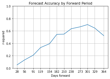
At short periods, up to 3 months, and particularly 1 month forward, we observe (see the chart below) mainly random noise with low out-of-sample r-squared readings (e.g., 0.04 at 28 days forward). As the forward period increases, up to around 273 or 301 days forward, so does the accuracy (out-of-sample r-squared around 0.60-0.70), before dropping slightly towards 364 days forward (0.50-0.60).
For additional information on the performance of the model, see the ‘Historical Performance’ section of the attached forecast;see also the historical performance commentary in the appendix.
Benefits
In general, machine learning algorithms do what equity strategy analysts should do. They are rigorous, don’t suffer lapses of concentration, consider all data, and recognize predictive combinations of conditions, and quantify the frequency and extent of those patterns in comparison to other patterns. The human brain is however quickly overwhelmed by so much data and often substitutes such a difficult question with a simpler one (attribute substitution bias). Additionally, confidence intervals can be easily calculated - another area where professionals struggle with their biases, typically overconfidence bias. Furthermore, the model incorporates new data with each new day, constantly learning from the extent of its successes and failures, reclassifying normal data ranges, and reidentifying patterns.
There are two further areas where our specific model has an advantage over humans or even other machine learning models. Firstly, we searched academic and professional literature to select the set of input factors, disgarding many as well, while equity strategy analysts might struggle to test the predictiveness of the variable combinations: lagging variables such as GDP and money supply are not useful. Secondly, while we apply machine learning in a standard way, a significant contribution to the model’s accuracy comes from the application of newer recurrent neural network (RNN) algorithms with these factors.
Finally, two anecdotal points encourage us. Firstly, the underperformance compared to benchmark of Renaissance Technologies’ longterm value fund indicates that even the leader in the field of machine learning models for shortterm trading is not yet filtering 6-12 month signals from the market. Secondly, that the majority of academic research continues to misplace its hopes in technical analysis (presuming that past actions of random and irrational agents contain useful information for predicting the future index returns). See reference [1] for a survey.
Despite these benefits, there are challenges when working with machine learning models. We present those in the next two sections.
Where We Are Cautious
Machine learning algorithms have a unique set of challenges, which require some adjustment from working with handmade human forecasts. Thus, we exercise caution in the following areas:
One of the main concerns is overfitting. Overfit models perform well on training data but fail to generalize well on new data. The similar accuracy scores between training and test data of our model indicate the model is not overfit. Furthermore, we do not tune hyperparameters, preferring to take default values or select reasonable values once according to the data. Moreover, we prefer a model based on a small number of economically relevant factors, rather than adding ever more factors.
To avoid concerns of data quality, we chose readily available, aggregated factors, which require little preprocessing or cleaning. Where normalizing data for backtesting, we only normalize over the data available at that point in time.
Complex algorithms may achieve higher accuracy, but transparency of the result falls. While we can show the sensitivity of the algorithm to changes in specific input factors, explaining the exact calculation for some submodels is not possible.
How well the model responds to new events depends to what extent the conditions match conditions which occurred in the training set, and the ensuing change in the index. For example, the conditions just prior to the index fall due to Covid-19 in 2020 were expansionary and there was no factor to indicate the ensuing pandemic hence the model forecast a rise in the index, which did not occur. Conversely, the conditions prior to the onset of the Ukraine war at the beginning of 2022 caused the model to forecast a drop in the index, and the index fell. When following the forecasts, we recommend first assessing if there are any unique circumstances which may not be analogous to the events present in the data since 1990.
We prefer to assess performance in terms of risk-adjusted returns when evaluating strategies against the S&P 500.
Finally, following a model requires a mindset to understand the model’s and one’s own fallibility. When the index follows the model’s forecast, all is good; if not, one needs to manage one’s doubts – which is easier said than done.
Key Risks
The key risks of a strategy following our forecasts relative to a long-only, passive S&P 500 strategy are:
Economic history does not repeat itself: the model does not recognize structural economic shifts and other novel events. That is, the factors we have selected and their particular combination are not mean reverting.
Animal spirits (market irrationality): The model forecasts rational economic index levels, but irrational agents maintain the index at different levels over a period longer than the portfolio’s investment horizon; or even, the model has been trained during a period of irrationality (from 1990 to now), but the economic conditions become rational.
The perceived accuracy of the model’s out-of-sample predictions is the result of luck; if so, the model will have no predictive power.
Competition with similar, but faster or more accurate models leads to underperformance.
How to Use It?
See the appendix for a sample forecast.
How to use it depends on your investment mandate and investment approach. We provide a recommendation for how each portfolio strategy type (long-or-short, long-or-cash, active) should position itself. Following the recommendation is not strictly necessary: simply heeding the recommendation when it is strongly positive or strongly negative is enough to improve returns. Similarly, the forecast may be used simply to determine the rate of contributions into a long-only strategy. Having a second, quantifiable, fundamentally based opinion to confirm or contradict your own opinion is invaluable.
Since these forecasts may struggle with novel situations (see ‘Key Risks’), we recommend following the forecasts during “normal” times, but to apply your own expert judgement during novel times. Our commentary also includes an assessment of the “normality” of the conditions.
The forecasts will be predominantly above zero so any strategy will be predominantly long. It will avoid obvious situations where fundamentals and sentiments have subsequently resulted in a market downturn.
Find Out More
We produce the forecasts monthly with a commentary on how to interpret and position each forecast. We can produce on request forecasts based on the last business day for unique situations. Contact us if you are interested to receive the forecasts.
We are interested to expand the forecasts to cover new indices and to improve accuracy with novel factors. Please talk to us about your ideas.
References
Jinan Zou, Qingying Zhao, Yang Jiao, Haiyao Cao, Yanxi Liu, Qingsen Yan, Ehsan Abbasnejad, Lingqiao Liu, and Javen Qinfeng Shi. “Stock Market Prediction via Deep Learning Techniques: A Survey”. 2023. 1, 1 (February 2023), 34 pages https://arxiv.org/pdf/2212.12717.pdf
Gunter Löffler. Equity Premium Forecasts Tend to Perform Worse Against a Buy-and-Hold Benchmark. 24 August 2021. https://www.uni-ulm.de/fileadmin/website_uni_ulm/mawi.inst.060/loeffler2022buyandhold.pdf
Eduardo A. Gerlein, and T.M. Mcginnity, Ammar Belatreche, Sonya Coleman. "Evaluating machine learning classification for financial trading: An empirical approach". February 2016. Expert Systems with Applications 54. https://www.researchgate.net/publication/292679922_Evaluating_machine_learning_classification_for_financial_trading_An_empirical_approach
Sai Krishna Lakshminarayanan, and John McCrae. "A Comparative Study of SVM and LSTM Deep Learning Algorithms for Stock Market Prediction". 2019. https://ceur-ws.org/Vol-2563/aics_41.pdf
Appendix
Sample Forecasts
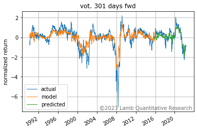
Training and Testing
The following chart shows the actual change in the index over 301 days and what the model achieved in training and subsequently predicted.
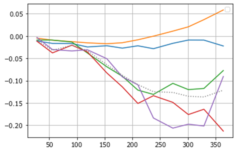
Submodel Forecasts
The following chart shows forecasts of each of the models, before weighting. The grey, dotted line is the combination of the submodels, weighted by their out-of-sample accuracy. The combination of models, even the less accurate models, improves the overall out-of-sample forecast accuracy.
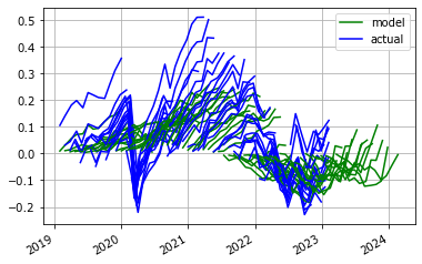
All Forecasts
This following chart overlays the forecast predicted each month ('model') and the actual change in the index from the date of the forecast ('actual'). A visual inspection suggests the forecasts predict the direction of the market well, but can understate the magnitude.
Historical Performance Commentary
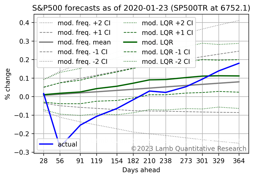
This section provides selected forecasts as would have been predicted at the time, only with data available, and overlays the index performance.
At the end of 2018, the model forecast above average returns. It was correct, but understated the magnitude of the returns.

At the beginning of 2020, the model predicted above-average returns. By the end of the year, it was correct due to a change in economic conditions, but it did not predict the shortterm price collapse due to Covid-19.
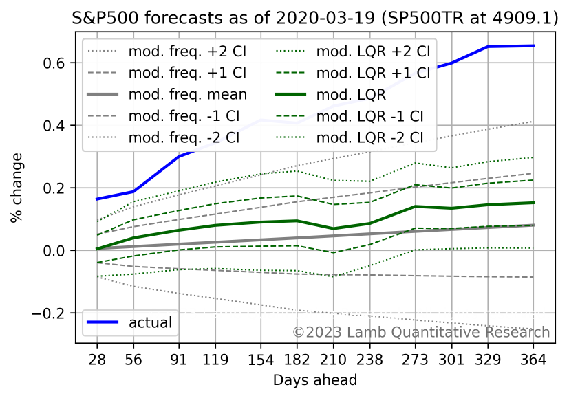
Following the price collapse from Covid-19, the forecast was for above-average returns. The forecast was correct, but understated the magnitude of the recovery.
The model correctly forecast the index returns for 2021.

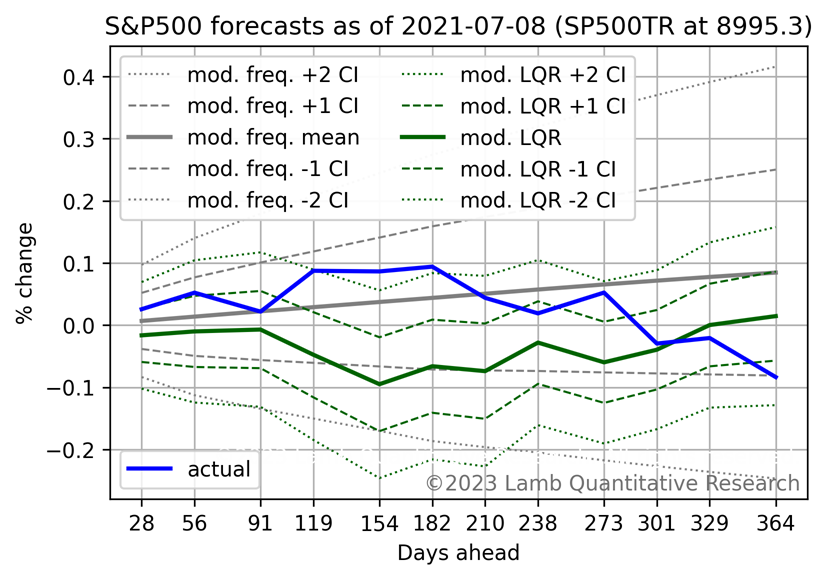
At the middle of 2021, the model predicted below average returns. It was eventually correct, but not before the market rallied toward the end of 2021, and then fell at the start of 2022.
At the end of 2021, the model was strongly negative, and this was correct.
In April 2022, after the index price fall at the beginning of 2022, the model was still negative. This turned out to be correct as well.

At the middle of 2022, the model was slightly negative, but indicated index levels would improve from the end of the year. This has been correct thus far.

Legal Disclaimer
The information contained in this white paper is for informational purposes only and does not constitute investment advice or an offer to buy or sell any security. Lamb Quantitative Research is a company registered in Switzerland and complies with the relevant securities regulations in that jurisdiction. However, the information in this white paper may not be suitable for readers in other jurisdictions, and Lamb Quantitative Research makes no representation that the information in this white paper is appropriate or available for use in other locations. The reader should not make any investment decision based solely on the information presented in this white paper. Investing involves risk, including the possible loss of principal, and past performance is no guarantee of future results. Before making any investment decisions, readers should consult with their financial advisor and carefully consider their own investment objectives, risk tolerance, and financial situation.
Copyright Statement
©2023 Lamb Quantitative Research. All rights reserved. This white paper and its contents are the property of Lamb Quantitative Research and are protected by copyright law. No part of this white paper may be reproduced, distributed, or transmitted in any form or by any means, including photocopying, recording, or other electronic or mechanical methods, without the prior written permission of Lamb Quantitative Research, except in the case of brief quotations embodied in critical reviews and certain other noncommercial uses permitted by copyright law.
Comments